

Architectural Energetics
Architectural Energetics: A Building Science Diary
Eight weeks of thermal comfort, daylight, noise and energy measurements from the University of Plymouth's Architectural Energetics module — the building-science groundwork behind how we think about older buildings today.
Please note all excel spread sheets used for calculations are included to the back of this diary, as an appendix.
Week 2 – 17.01.05
L1 - Measurement of Thermal Comfort, and some energy considerations.
Introduction
It was our task to measure the different types of thermal comfort in different areas. The types of measurement that we took were:
Wet bulb temperature;
Dry bulb temperature;
Air speed; and
Mean radiant temperature.
The areas in which we took these results were:
Technical library – central desk;
White box – corner at the front of the theatre;
Canteen – corner by the window; and
Outside courtyard – under the “arcade” - raining.
Method
The method used is as described in File 1. Module booklet 0405.doc L11
To measure Mean Radiant Temperature a globe thermometer is used.
To calculate Wet and Dry Bulb Temperature a whirling hygrometer is used.
To calculate Air Speed velocity in metres per second a Kata thermometer is used.
Results
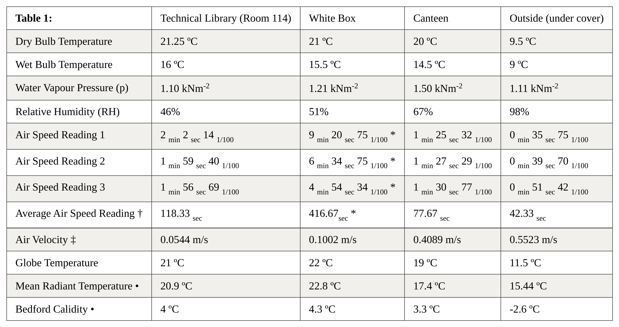
NOTES:
* A star denotes use of the thermometer with a cooling factor of 532. Cooling factor for other tests were carried out using thermometer with a cooling factor of 537.
† For the purposes of calculating average air speed one hundredths of a second were rounded up where necessary.
‘p’ is found by cross referencing Wet and Dry bulb temperatures onto the Psychometric Chart2.
‘RH’ is found by cross referencing Wet and Dry bulb temperatures onto the Psychometric Chart3.
‡ Air Velocity in m/s is found by using the Air Velocity by Kata sum4.
The Technical Library and White Box are both assumed to have an air velocity of 1.0 m/s or less. The Canteen and outside are both presumed to have an air velocity greater than 1.0 m/s.
• The values for mean radiant temperature and Bedford Calidity are found by using the Caladity spreadsheet5.
Conclusion: (See appendix 2)
From the above table I can deduce that the White Box is the warmest and stuffiest area. I know this because the air speed is very slow; hence the reason it took on average 416 seconds to cool down. Also it is the warmest area studied; this is almost certainly due to the low air change rate per hour. These two main factors have the result of pushing the Mean Radiant Temperature up to 22.8 ºC and the Bedford Calidity up to 4.3 ºC. Both of these values are the warmest temperatures measured in our series of tests and it is not surprising that it is sometimes difficult to stay awake in lectures – there is a severe lack of oxygen / fresh air in the room!
The Technical Library is a much better work place than the white box as it has slightly lower temperatures overall. It is a pleasant area to work in as can be seen by the Bedford Calidity temperature of 4 ºC. This number is considered to be perfect, and is probably due to the fact that the Technical Library has a series of windows along one wall – something that the white box is drastically missing. I know that the windows are responsible for helping to cool the room because the average air speed reading is almost 4 times smaller than that of the white box – proving that there is a breeze entering the room.
The Canteen is slightly cooler than the two previous rooms – its Bedford Calidity is 3.3 ºC, this is “comfortably cool”6 and is obviously because this is a very open space with one wall almost entirely glazed. The area is open to the Gallery at one end, with no door, also the door to the First Years Studio is constantly in use and there is a steady flow of people in and out to the (external) courtyard. All of these factors along with the amount of glazing reduce the Air Speed Rating drastically: to an average of 77.67 seconds. Another observation that can be made in the Canteen is that of the increased Relative Humidity compared to other indoor rooms, this is most likely due to an external door that is constantly in use and steam and vapour from the kitchen. All of this will push the RH up – effecting the Mean Radiant Temperature – and keeping it down to a lower than average value of 17.4 ºC (where other rooms were roughly 3 - 4 ºC higher than this).
It is not surprising that Outside the Bedford Calidity is -2.6 ºC. This does not mean that the temperature outdoors is -2.6 ºC – otherwise everything would be freezing! What it states is that it is “much too cool”7 and anyone outside would probably need a coat and scarf. This is understandable considering it is mid January and the Globe Temperature and Mean Radiant temperature were 11.5 ºC and 15.44 ºC respectively. The wet and dry bulb temperatures are very low outside, this is due to a combination of the low temperature and light rain that we were experiencing at the time, and this also accounts for the high RH value of 98%
Week 3 – 24.01.05
S1 – Explore heat loss from a building and use thermal comfort meter software.
Part 2
Introduction
It was my task to experiment using the “Thermal Comfort Meter” and “Energy Balance and ASF%” spreadsheet to explore the different factors involved in producing a comfortable room.
Method
The method was as described in File 1. Module booklet 0405.doc S18.
I explored using the “Thermal Comfort Meter” software and tested different environments and activities and different temperatures. Noting the main changes within these parameters; the results can be seen in table 2.
Part 1: Results
Table 2:
Conclusion: (See appendix 2)
From table 2 it can be seen that gender has no effect upon dissatisfaction of thermal comfort in an area or room. Another conclusion I can make is that a room that has fewer than 10% of people dissatisfied is a reasonable environment.
The type of work being conducted drastically lessens the thermal comfort of a room, for example column 4 on the “HOT” table shows work load increased from “physical exercise” to “heavy exercise” – and this increases the amount of dissatisfied people from 60% to 91%
Relative humidity does little to effect the thermal satisfaction of people in an area. This can be seen from “AVERAGE” table, column 4, and “HOT” table, column 2. In both cases the RH is increased or decreased by about 20% and the only effect is to satisfy or dissatisfy 2%-3% of the people.
The main factor that improves or worsens thermal satisfaction is the Temperature (ºC), changing this value by only a few degrees has a massive effect on the percent of dissatisfied people.
Air movement in a room can help cool people quite well. This can be seen in the “office scenario” from the “AVERAGE” table. This justifies the case for mechanical ventilation of a room – though a lot of power is often used in mechanical ventilation it is more than worth it because of the amount of people that it satisfies.
Week 3 – 24.01.05
S1 – Explore heat loss from a building and use thermal comfort meter software.
Part 3
Introduction
It was my task to experiment using the “Energy balance” spreadsheet9; using this I must input data from my Integrated design project, to calculate simple thermal performance of a sketch design scheme.
Method
Using data from my design I estimated amount of wall area, window area, size of building, number of people etc. I would use the spreadsheet twice to calculate heat-loss, passive solar gain, ventilation, fenestration and envelope construction in the Winter and the Summer.
Results
Table 3:
Summer Time:
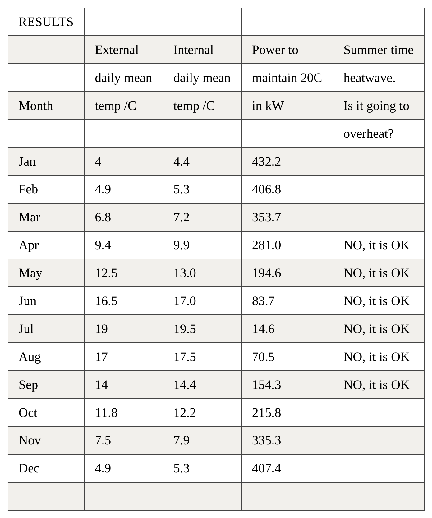
Table 4:
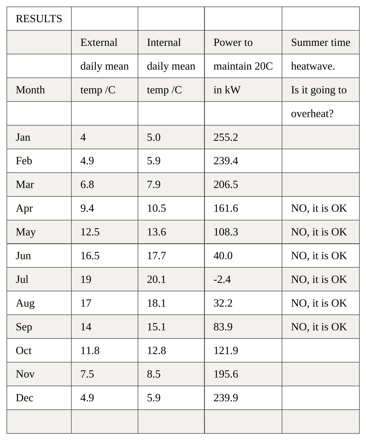
Winter Time:
Conclusion
During the summer indoor temperatures seem to be quite reasonable, during May, June, July and August they are below 20ºC which I see as a good thing because during these months the temperatures are normally quite hot. This results in the overheating of buildings, so for a building to be slightly cool during the summer would create a nice effect. The reason that the building is well cooled during the summer months is because of the effect of circulating air and ventilation. This is achieved by using large expanses of glazing that can be opened; this provides a high Air Change rate per Hour (ac/hr). Only small amounts of power would be needed to help warm the building in April, May and September.
In the winter months of December, January, February and March the amount of heating required seems to be excessive. I would estimate that below 200 kW to a reasonable amount to use to heat a building. I believe that the amount of energy required to heat the building is slightly great because of the expanse of windows I have used. This will affect my design and I will amend my design accordingly. However, changing the windows in my design will also affect the natural ventilation rate and could increase the temperature in the summer – this is an effect I must consider.
Week 4 – 01.02.05
L4 - Simple environmental noise measurement
Introduction
It was our task to measure different frequencies and noise levels of various noise and sounds and to draw conclusions from our findings. The types of experiment that we conducted were to:
Compare external and internal sound levels;
Investigate noise levels associated with different sources;
Explore the change in noise level over distance;
Determine sound pressure levels in each octave over the frequency range; and
Measure noise transmission across an element (door).
Part 1 & 2
Method
The method used is as described in File 1. Module booklet 0405.doc L410
To measure sound pressure levels in dB(A) using a simple sound level meter, the B+K type 2232. NB dB(A) is different to dB, where they represent a measurement of sound as if heard by a human ear, and measured by an electronic device, respectively.
Results
Table 5:
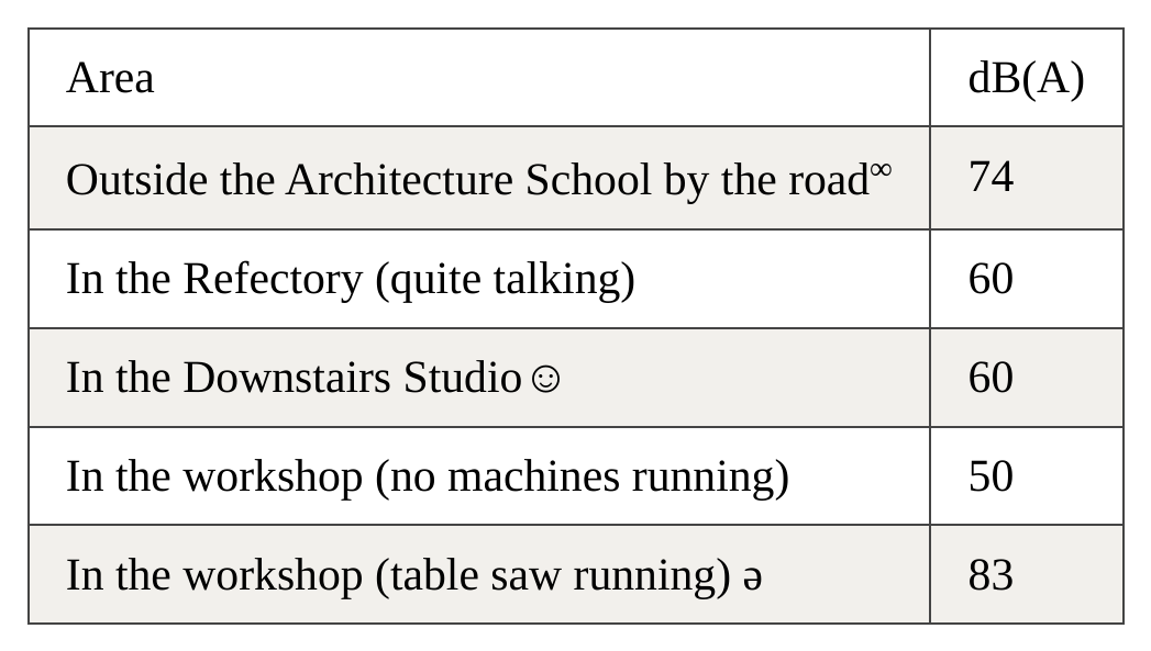
∞ NB the reading was taken directly opposite the building site on Notte Street, immediately outside the front door of the School of Architecture. The building site would have altered and increased all noise measured.
☺Take note that a TV was in operation in the studio and this is not a normal activity, this could increase the noise level recorded.
ә The reading taken here was taken while saw was running, but NOT cutting wood; when cutting wood the saw is a lot louder.
Conclusion
From these results I can see that a normal “working space” (e.g. a space that is used to work in – a studio, office or classroom) has an average sound level of 56 dB(A) (NB decimal decibels are never used)11.
The noise of a building site next to a road produces 74 dB(A), and in my experience I would say this is quite quiet. The site near the Hoe Centre is relatively quiet compared to most building sites in that there is no excavation, demolition or heavy machinery used. At the moment the only loud noises from the site are that of lorries or the “clank” of steel as the frame is erected. However it is easy to see how noise pollution from such areas could cause a major problem in residential areas.
Noise produced from heavy machinery (the table saw) in the workshop is very loud. It is the loudest single noise that we measured and it is fully understandable why regulations recommend the use of ear protection! Long periods of time with exposure to noises of this level have been proved to damage hearing. While noises above 100 dB(A) create a “temporary threshold shift” (meaning “a ringing in the ears and inability to only hear loud noises for a short time”) which temporarily deafens a person, loud noises below this level do not. It is for this reason that a person may not notice their loss of hearing until it is far too late and the damage is already done.
Part 3
Method
The method used is as described in File 1. Module booklet 0405.doc L412
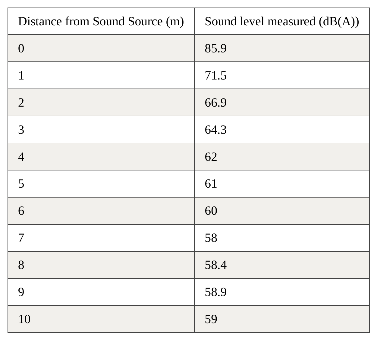
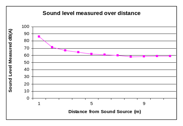
To measure sound pressure levels in dB(A) from a B+K sound source as a function of distance (at 1M intervals), using a simple sound level meter, the B+K type 2232.
Results
Table 6:
Graph 1:
Conclusion
From Table Six and Graph One I can see that at a distance of 3 metres the speed at which the sound level decreases is greatly slowed. The sound level soon levels out at around 60 dB(A) and then at a distance of 8 metres it actually begins to rise in sound level. From 8 to 10 metres the increase is only slight but it is defiantly a noticeable rise, this is due to the reverberance of sound from side walls and (mainly) the back wall. Often cases like this can actually make it harder to hear at the back of the room than one may expect than one might expect. This is because even though the sound being heard may be louder, the noise heard has been bounced from the wall behind the listener – and thus, been heard again – this can produce poor sound quality and create a slight echo.
Part 4
Method
The method used is as described in File 1. Module booklet 0405.doc L413
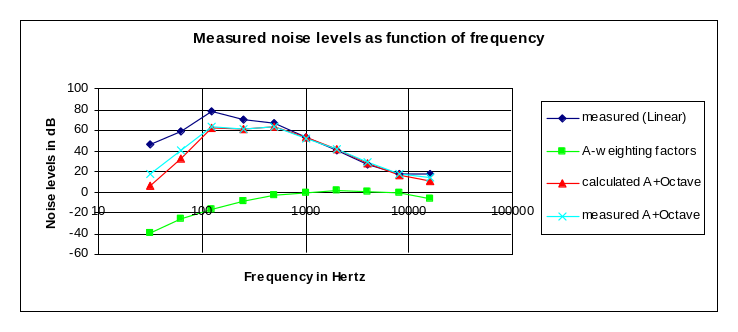
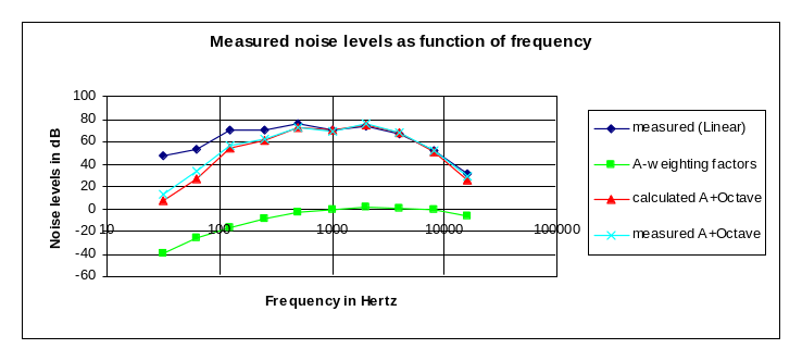
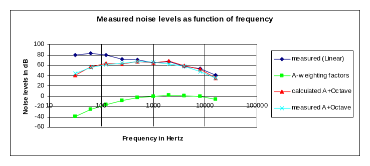
To compare various Sound Pressure Levels in dB and dB(A) using B+K SLM. This was conducted three times, once for “Pink Noise”, once for “White Noise” and once for “Traffic Noise”.
Results
Graph 2:
Pink Noise –
Graph 3:
White Noise –
Graph 4:
Traffic Noise –
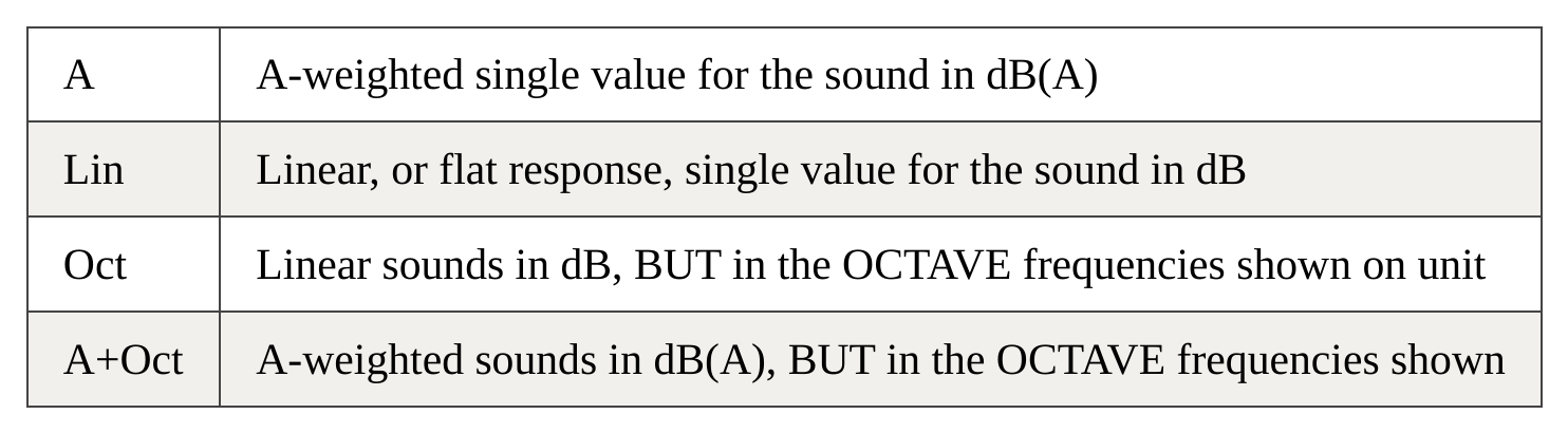
Legend14:
Conclusion
From Graphs labelled 3 to 5 I can deduce that between 1000 and 1000 hertz white noise sounds louder than pink noise, of course this is not really the case because at no time has the volume been altered. The measurement reading is measuring a louder noise because it is taking into account the effect that a human ear has upon a sound, this means that we sometimes here sounds differently than they are actually being played. This is a good example of why we sometimes need to measure a noise using an electronic scale of dB, not dB (A).
Traffic noise is loudest at lower dB level. This means that it is made up of more low tones, and less high tones, this would account for the sound of a truck rumbling by or lorry passing outside and it still being audible indoors. The noise generated is a low frequency (between 0 and 100 hertz), these noises carry easily through building elements with a great mass, concrete floor slabs, block-work walls and the like.
NB White Noise is noise made up of ALL frequencies; Pink Noise is noise with the high and/or low end bass removed.
Measurement of dB as a linear number is a scientific measurement.
Octave measurement measures different frequencies as well.
While doing these 3 tests the Lab door was open (room 114) – some sound may have escaped through here, and background noise could have entered.
Part 5
Method
The method used is as described in File 1. Module booklet 0405.doc L415
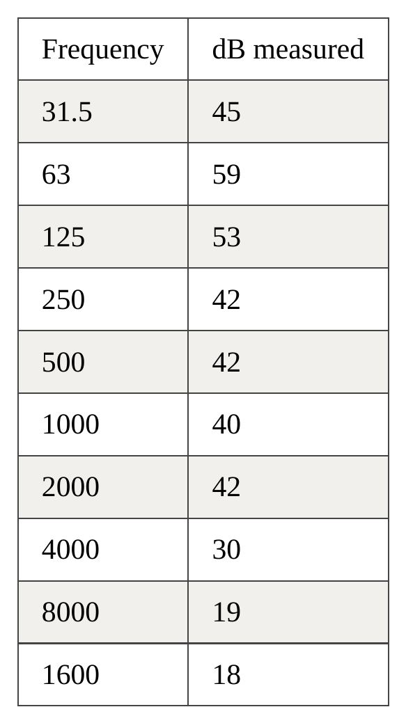
To measure sound pressure levels in dB(A) using a simple sound level meter, (the B+K type 2232) through a building element. The building element that we chose was a wooden door, with 2 glazing panels above it, and no draught seal around the edge. Results were recorded then input on the excel spreadsheet16.
Results
Table 7:
Sound measured next to the sound source
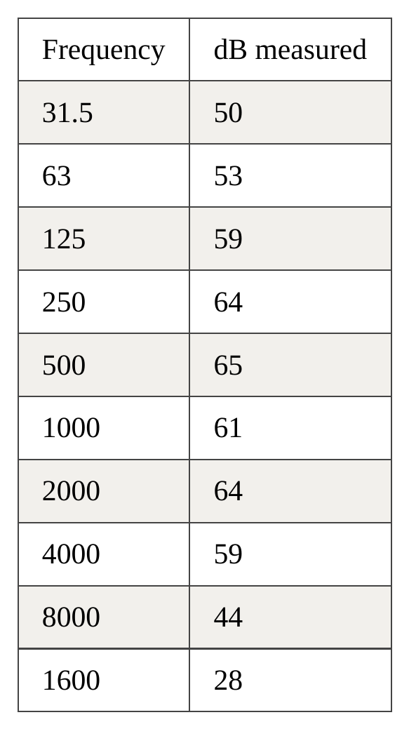
Table 8:
Sound measured through a door
Conclusion
From the two tables above we can see that clearly the door has a good sound insulation rating. The average Sound Reduction Index (SRI) measured was of 16.3. The noise level drops through the door were of 11dB and dB(A). This is quite a good RSI and drop in sound level but it could be greatly removed by filing the air gaps around the edge of the door. This could be done using an insulation tape or draught excluder. Also the two windows above the door probably allow sound through a lot easier than the walls do – if these windows are not necessary then they could also be removed and filled with the appropriate wall material (stud partition or brick/block work).
From the graphs in “DIARYFile8.Noisetransmission.xls” I can see that sound is only really heard through the door between about 1000 hertz and 8000 hertz. This means that the door successfully blocks sound transmission at all other frequencies. At a glance this may seem like the door is doing a good job and insulating against unwanted sound, however the fact that the human ear cannot hear very high and very low frequencies needs to be taken into account. The sounds that are not passing through the door probably cant be heard by the human ear anyway! The door is not very good at sound proofing against low sound levels and this is probably because these sounds travel well through a dense material. This may mean they are “rumbling” through walls and floors as well as the door. To prevent these sort of sounds padding could be used, this helps dampen a sound, for example a “bass box” or “subwoofer” of a stereo system could be placed on stilts or a padded base so that the low end frequency sounds are not carried through the structure of the building and causing unwanted sounds in other rooms.
Week 5 – 13.02.05
S4 – Understanding dB(A) to dB conversion, SRI, reverberation timing, and natural ventilation and acoustics.
Introduction
It was my task to measure various types of sound levels, frequencies and noise levels and to draw conclusions from the graphs and results found. The software used and tests conducted were to:
Compare dB(A) and dB;
Calculate area weighted acoustic absorption coefficients and RT17;
Sound reduction Index (SRI) for complicated elements of buildings;
Speech intelligibility through and element (door);
Speech intelligibility in an open plan area; and
Calculation of natural ventilation & acoustics.
Part 1
Method
The method used is as described in File 1. Module booklet 0405.doc S418
To directly compare dB(A) (as heard by a human ear, and dB (as measured by an electronic device).
Results
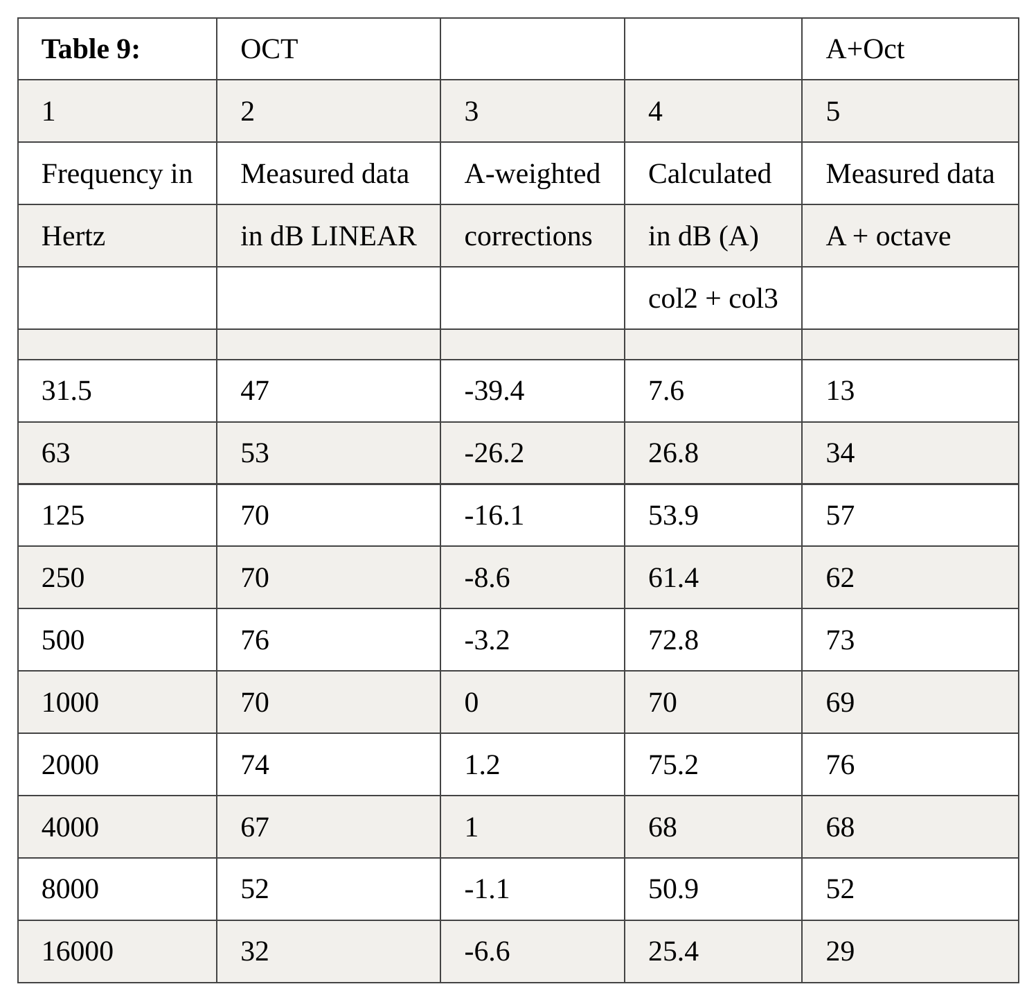
Column 2: dB linear, is a sound level measured by an electronic device, in this case the B+K precision sound level meter.
Column 4: shows the measured dB sound levels converted into dB(A) – as if a human ear was measuring them.
Conclusion
As can be seen the human ear measures different frequencies at different volumes. This is much the same as the B+K precision sound level meter, except that results are more extreme – for example some sound levels calculated in dB(A) are far quieter than when measured using the B+K precision sound level meter.
This definite drop in sound levels is seen to be at its greatest (lowest drop) at frequencies of 16000, 250, 12563, and 31.5. From these results we can clearly see that the human ear cannot pick up these frequencies very well, as has trouble hearing them. Also at frequencies of 2000 and 4000 the dB(A) calculated is actually greater than that measured by the B+K precision sound level meter – this means the human ear is more receptacle to these frequencies, and thus, measures them at a louder dB(A). From these results we can clearly see that the human hearing spectrum is best between 250 hertz and 4000 hertz. An interesting experiment may be to measure frequencies that can be heard from different age groups, and to plot the results.
Part 2
Method
The method used is as described in “File 1. Module booklet 0405.doc S4”19
To calculate the area-weighted acoustic absorption coefficients and the reverberation times as a function of frequency for a classroom. Absorption coefficient values were taken from “Acoustics in education” book.20
Results
See excel sheet – “ENBS diary File 6. Acoustics RT, SRI and SPINY.xls” and below:
Graph 5:
Conclusion
As you can see the reverberance time is greater for frequencies of about 100 to 300 hertz. Normally the greater the reverberance time the worse the room is for acoustics, this is because if the reverberance time is too great a very distracting echo will be created and the intelligibility of speech will be difficult. As the experiment indicates this test conducted was for a classroom where reverberation could cause quite problem. Some ways in which reverberation times can be reduced are:
Close curtains;
Use soft materials on the walls;
Break up large flat surfaces with a textured material such as wood;
Thick carpets used not shiny floors.
Part 3
Method
The method used is as described in “File 1. Module booklet 0405.doc S4”21
To predict the noise transmission through a complex element in a building using data from my “House of the Elements” project and the software spreadsheet “File 6”22.
Results
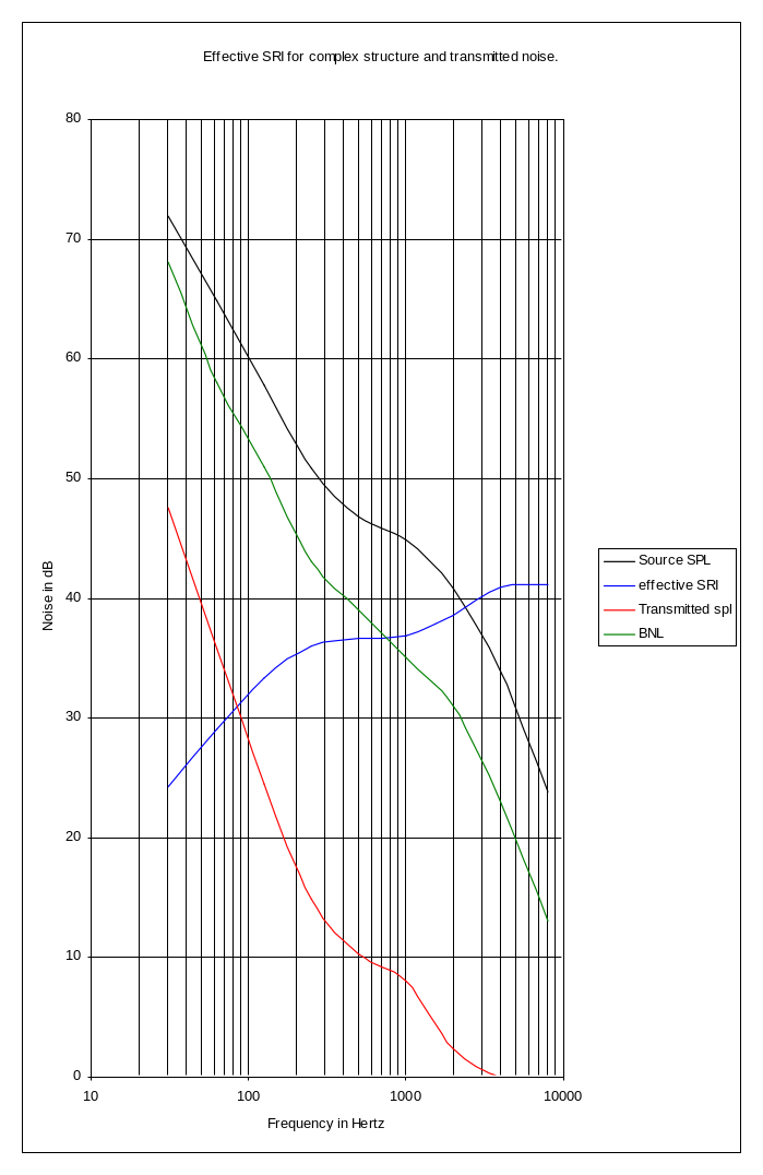
Graph 6:
Conclusion
Graph 6 shows that the transmitted noise is not always less than the BNL 35dB curve. On this criterion, the complex wall would normally not be acceptable. The noise level does reach beyond 35 dB at a number of occasions and the SRI will need to be improved. This is due to the workshop (taken as “Music room, drama space, music practice room” - to calculate appropriate sound level) being close to the classroom. I will probably have to redesign this area of my room layout for my “House of the Elements” as the sound level reaches well beyond 35 dB, and even into the 40 dB area, which is unacceptable.
Part 4
Method
The method used is as described in “File 1. Module booklet 0405.doc S4”23
To calculate speech intelligibility through a door using data from my “House of the Elements” project and the software spreadsheet “File 6”24.
Results
Graph 7:
Total Dot Score = 1825
Conclusion
Since the dot field score is 18, this is distracting and the spaces would NOT be acoustically private. This is due to an air gap of 0.005m*m around the door!
Part 5
Method
The method used is as described in “File 1. Module booklet 0405.doc S4”26
To calculate speech intelligibility in an open plan area using data from my “House of the Elements” project and the software spreadsheet “File 6”27.
Results
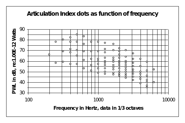
Graph 8:
Graph 9:
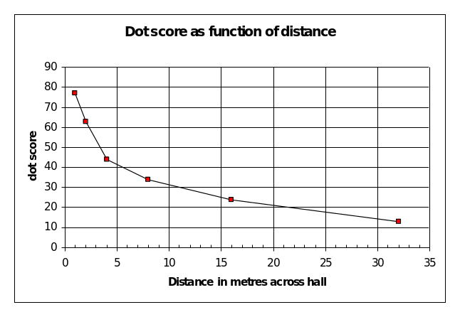
Total Dot Score = 4128
Conclusion
A “Dot Score” of 41 in an open plan area provides ‘good communication’, see Table 10 below:
Table 10:
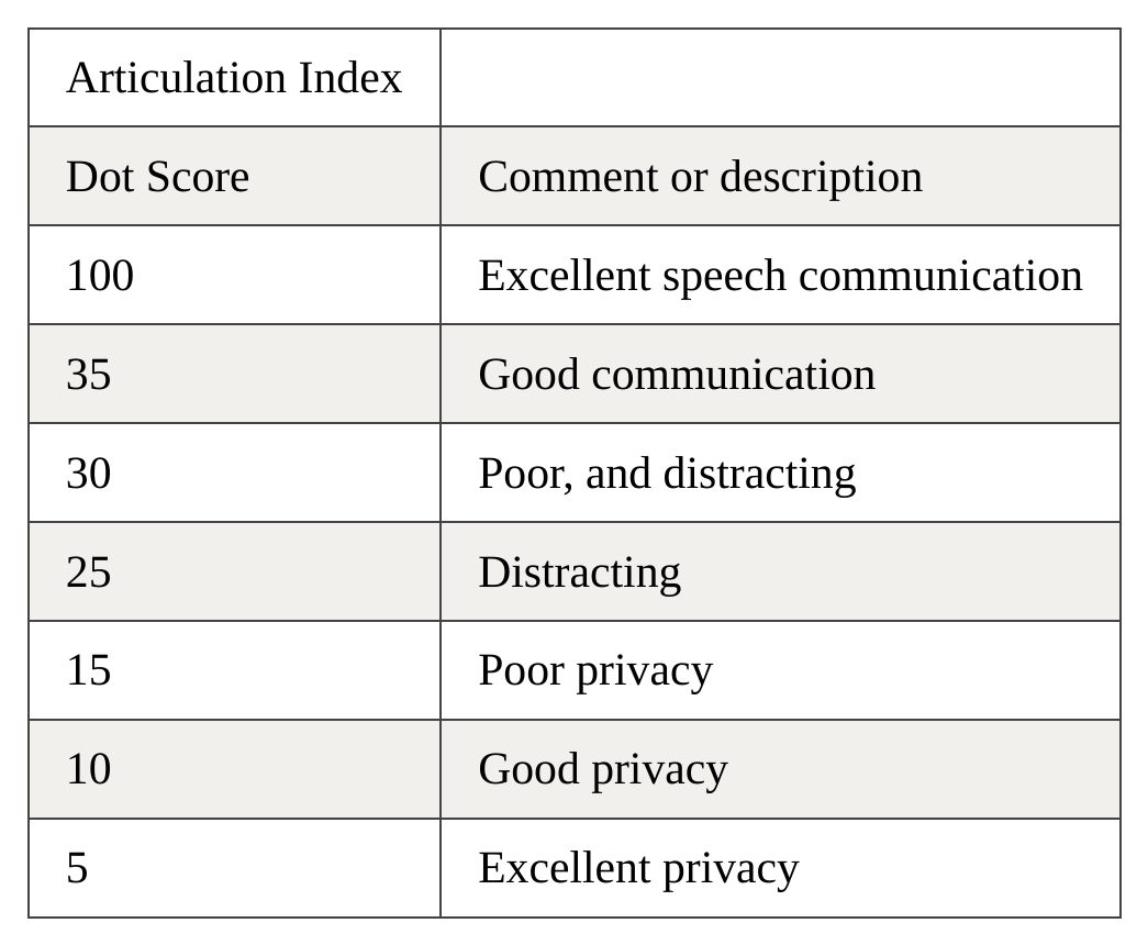
As we can see, in an open area any dot score of above 35 is a good result, however the dot score of 41only applies up to a distance of 5 metres. Up to a distance of 10 metres the dot score is approximately 32, which is still a good value, but at distances over 15 metres the noise becomes poor and quite distracting. This open plan room would only be reasonable where the distance in metres for reasonable communication were below 10.
Week 6 – 14.02.05
L3 – Skylight distribution in a real room.
Introduction
It was our task to measure the different illuminance/luminance of natural light falling on surfaces and to draw conclusions from our findings. The types of experiment that we conducted were to:
Measure the distribution of natural light in a room;
Compare the luminance of different materials; and
Calculate the ASF%29 for “The House of the Elements”.
All measurements made were done by using the “Hagner Universal Photmeter”, this is a light meter capable of measuring incident flux falling on a surface, the illuminance, and the reflected flux from a surface, the luminance.
Part 1
Method
The method used is as described in “File 1. Module booklet 0405.doc L3”30
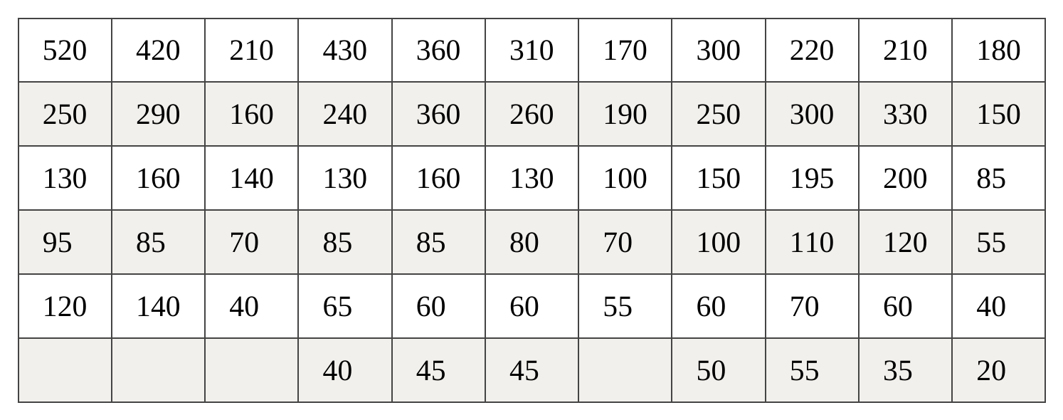
To calculate the natural light distribution across a room we decided to use room 115 as this has an excellent arrangement for this experiment. We set out a grid of chairs at 75cm centre to centre spacing and took a reading at the centre of each chair.
Results
Approximate layout of room 115 with horizontal luminance in lux measured at centre of each chair:
Table 11:
WINDOW 1 WINDOW 2 WINDOW 3
1.2m Window. 0.8m 2.5m Window. 0.5m 2.5m Window. 0.7m
Column. Column. Column.
8.2m Overall Length
1.2m Window.
Height of Room = 2.8m
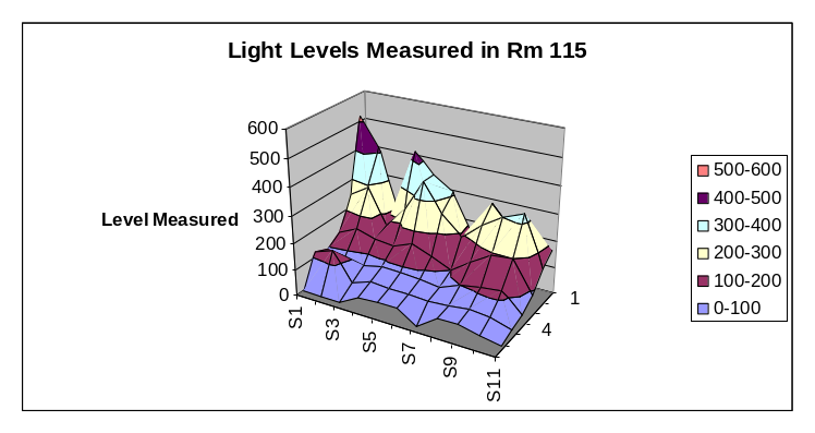
Graph 10:
Conclusion
When the table and graph are compared it can easily be seen that the highest lux levels are next to the windows. The back window has a relatively low lux level rating in comparison to the other 3; this is because it is a North facing window. The other 3 windows are south facing and thus let more light in.
Window 1 had the greatest lux level, this could be due to shadow that buildings outside create. As we get closer to the front of the room (where the door is) it gets gradually darker. The window on the north facing wall could be affecting the light lux level of Window 1.
Part 2
Method
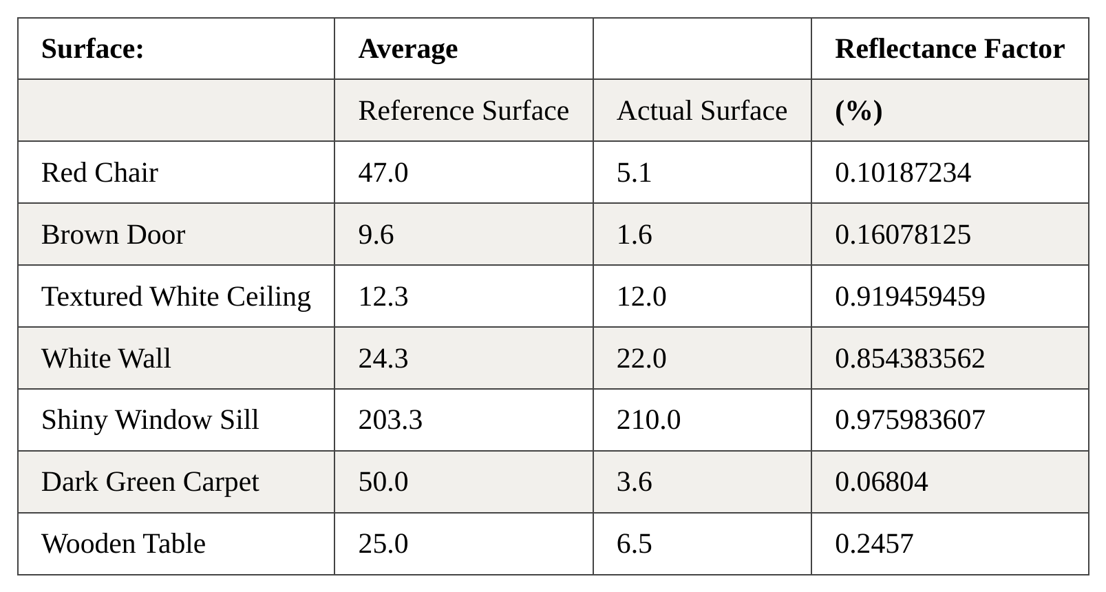
The reflection factors of surfaces were obtained by measuring the reflected flux from that surface and comparing it to the reflected flux from a standard surface of known reflectance, R. The reflection factor of the surface can be calculated using the equation31:
Reflection Factor (%), R = Rs*Ls / Lr
Where:
(1) Ls the luminance in cdm-2 of the relevant surfaces, for example the red cover to one of the chairs,
(2) Lr the luminance in cdm-2 of the reflection reference plate. You will see that the Hagner reflection reference is quoted as Rs = 94.5%, which we write as 0.94532.
Results
Table 12:
Conclusion
By making 3 tests for each surface and calculating the average value the most accurate reflectance factor could be calculated. As can be seen, not surprisingly, the “Dark Green Carpet” is the worst material at reflecting light. However, this is not necessarily a negative point because in a lecture room (such as Room 115) a shiny reflective floor could hinder learning by distracting pupils. Sometimes shiny, light floors may required, such as in dance halls or sports facilities rooms. The “Shiny Window Sill”, “Textured White Ceiling” and “White wall” all have almost exactly the same reflectance factor, this is most likely because they are all painted white – which reflects light extremely well.
Part 3
Method
To use “ENBS Diary SUMMER - File 2. Energy balance and ASF% .xls” spreadsheet to calculate the ASF% of my Visitor centre and to draw relevant conclusions. Materials specified to be used were similar to those of room 115.
The room that I will use in this example has a total surface area of T m2 which includes the four windows of area A m2, and decorated to achieve an area‑weighted reflection factor R. If the windows are glazed with optical transmission factor t and the vertical angle of available sky at the centre of the window is v, then the average skylight factor percent, ASF%, following the Sumpner‑Lynes‑Crisp method, is given by,
ASF% = t v A / T (l – R2)
For the room in this discussion, the total surface area is 2080 m2, which includes all of the windows of area 60 m2, and the room is decorated to achieve an area‑weighted reflection factor 2.06 If the windows are glazed with optical transmission factors of 0.85 and the vertical angle of available sky at the centre of the window is 300, then the average skylight factor is calculated to be 2.53%.
As this number is between 2% and 5% the room can be described as “bright and cheerful” and would not require any further attention as far as natural lighting was concerned.
Results
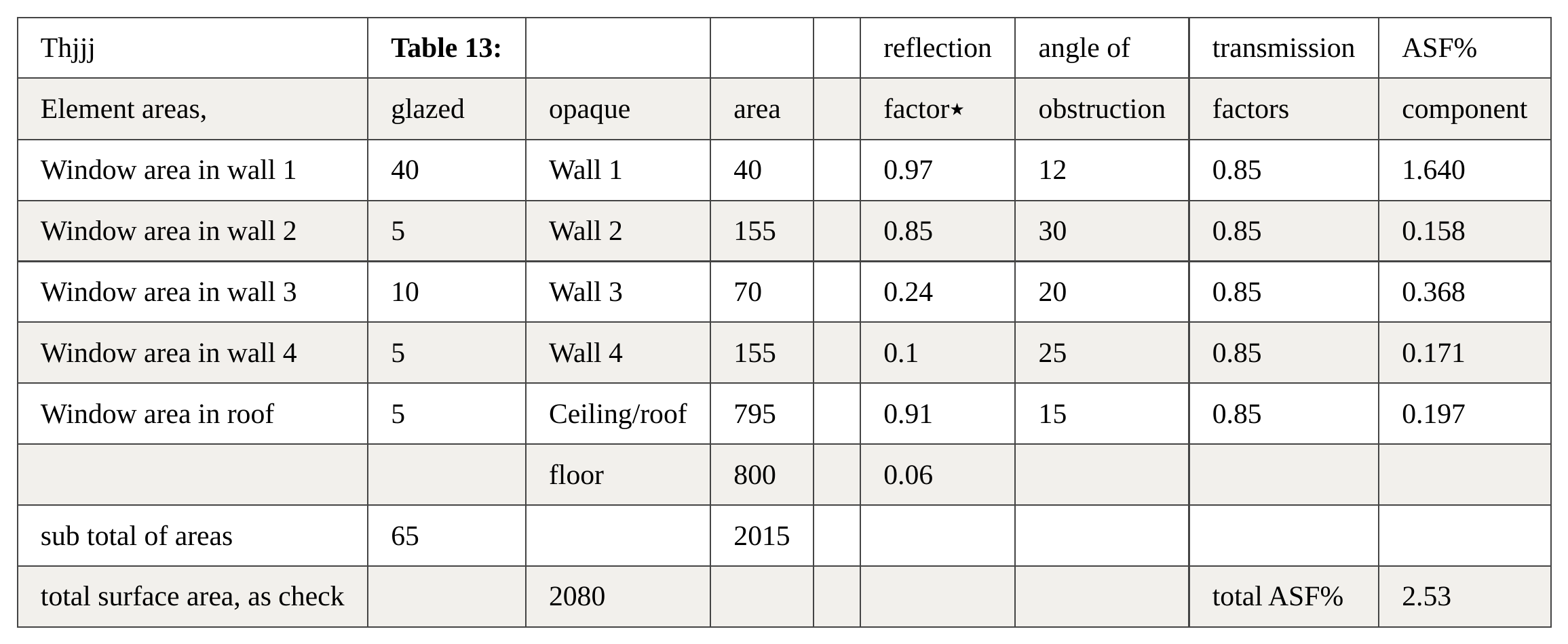
٭ Materials used were as Room 115: Wood, Dark Green Carpet, Red Fabric, White Paint, Textured White Paint, and Shiny White paint.
Conclusion
My room is O.K, but could be improved. The floor could be given a slightly lighter shade, and the wood panelling on one wall could be replaced with paint or a lighter wood. Either this or the finishes on the surfaces could be rotated, for example darker surfaces on the smaller areas. So the reflection factor of 0.24 (wooden panelling) could be placed on Wall 1 instead of Wall 3, the reflection factor of 0.1 (red fabric) could be placed on Wall 3 instead of Wall 3, and so on.
Week 7 – 21.02.05
S3 – Predicting iso-skylight factor contours using “nimbus”.
For this task I was meant to be able to load a piece of software called “nimbus”, however, after following the instructions set out in the Module booklet – Part S333 I was confronted with the following errors:
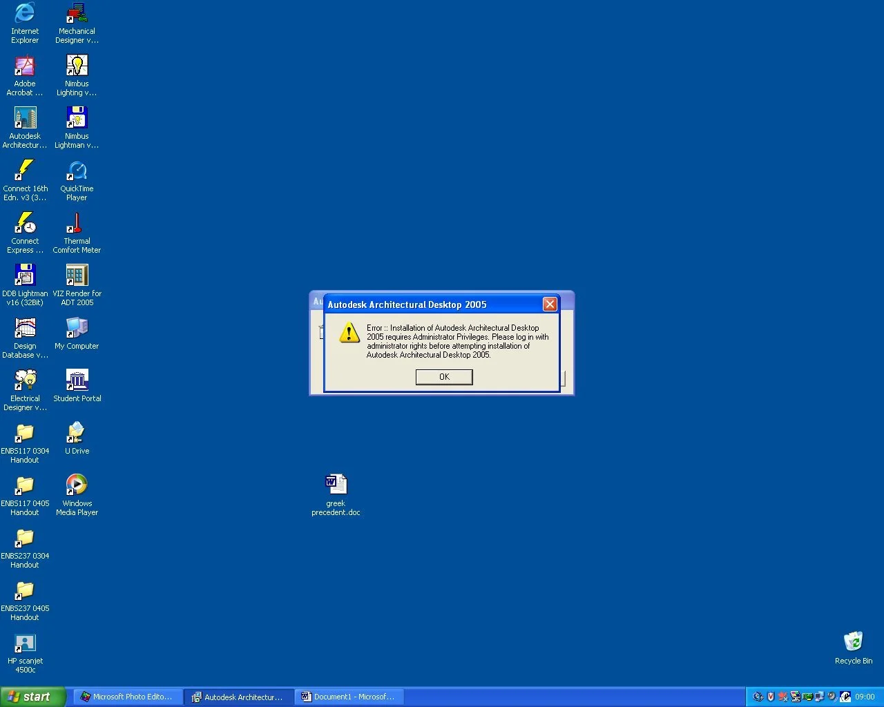
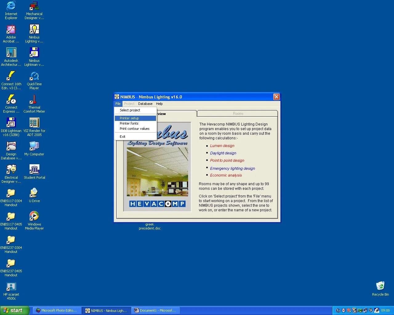
As a consequence I have been unable to proceed with this self learning experiment. Please accept my apologies.
Week 8 – 05.03.05
L2 – Introduction to Lighting, and light Measurements.
Introduction
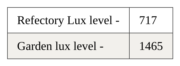
Our task was to measure light levels in various areas of the Hoe centre, 2 sets of measurements were taken in two areas, to measure the amount of natural and artificial lighting in a room and the effects that these lights have.
Method
To use measure the light levels in the following areas:
The refectory;
The rear garden;
The lecture theatre (White Box);
The studio; and
The basement corridor.
A series of graphs were produced to display these results34.
Part 6
Using the Minolta T-10 lux meter my next task was to compare the light spectra of the following items:
GLS lamp,
Fluorescent tube,
Low pressure sodium lamp, and
Skylight.
The different effects of these various light spectrums were then photographed.
Results
Part 1 & 2
Table 13:
Part 3
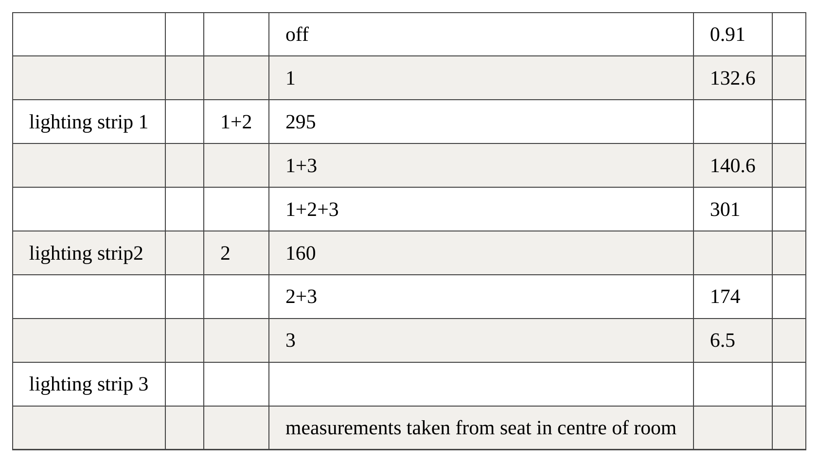
Natural and Artificial Lighting in the White Box:
Table 14:
Conclusion
As can be seen when all lights were off in the White Box there was still a lux level of 0.91 – this is relatively high for what seems to be a dark room. However on closer inspection it can be seen that small amounts of light can filter through the covered windows, also 2 doors were left open in the room – hence the lux level of 0.91.
When all lights are turned on the total lux level is 301, I am surprised this is not slightly higher, but when the height of the ceiling is taken into account (it is very high so lights are far away) its not surprising that the lux level is not higher.
Part 4
Stage 2/3 Studio - room H326
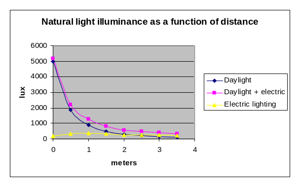
Graph 11:
Conclusion
As can clearly be seen at a distance of 0M from the window the lux level is 5170 with the artificial lighting on, and 4970 with it turned off. This is very high and is probably because the windows are very large in this studio and the sun was shining. The graph steeply curves until a distance of about 1.5M where it levels out at around 400 lux with the lights on, and 200 with them off. Clearly it is a very good idea to sit close to the window if natural lighting is important. As a studio was chosen for our study it is a shame that natural lighting doesn’t reach further into the room as natural lighting can be an important factor when using paints or pastels to produce high quality art work.
It is strange that the artificial (electric) lighting level changes from around 300 lux to 250 lux. This could be due to obstructions in the studio creating shadows, or the efficiency of each lamp varying. I.e. newer lamps (that have just been replaced) will have a higher lux output, also the maintenance (cleanliness) of a lamp effects the lux level output of a lamp greatly.
Part 5
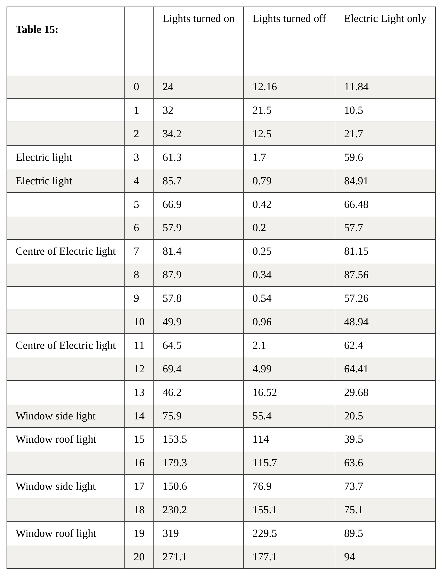
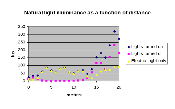
Measured light levels in the Basement corridor.
Graph 12:
Conclusion
This set of results is rather more varied than before, this is because of the various types of illumination that are in effect in the basement. There are a series of roof lights, high (small) windows, and artificial lighting.
The measurements were taken form the back wall (against the workshop) and measured travelling towards the stairs, as can be seen the closer to the stairs the measurements are taken the greater the lux level. This is because of the 2 large roof lights and the side windows. They greatly increase the amount of lux measured.
The artificial lighting level varies slightly because of “extra” light coming from around the corner in the basement, also I noted that many of the plastic cases that cover the lamps were yellowed and old, this can greatly decrease the output of the lamps, also the covers were dirty.
At around 6M with the artificial lighting turned on a light level of 57.9 lux was measured, this is almost 50 lux, which is the required amount for an art gallery. I was surprised to find that 50 lux is actually quite dark for the viewing of art work, if a client required a higher lux level (eg 100 lux) then paintings (especially watercolours) would only be allowed to be displayed for half the amount of time due to the increased lux level being shone on them. This has had quite an effect on the “Hour of the elements” Gallery design as I was worried about inadequate lighting levels. After seeing 50 lux for myself though I am now confident that the windows I have positioned (high up, narrow lights) will be more than sufficient for the display of art work pieces.
Part 6
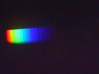
GLS lamp:
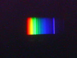
Fluorescent tube:
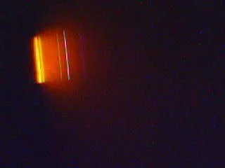
Low pressure sodium lamp:
Skylight:
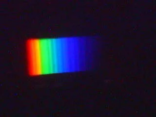
Using the Minolta T-10 lux meter I looked at the above four lighting sources. As can be seen the “skylight” has the best colour spectrum as it clearly shows every colour – not only does it show each colour though, it shows them all very well.
The “fluorescent tube” spectrum is similar to the “daylight” spectrum except that is has clear bands in the green and blue areas. The blue band is quite defined and this is probably because 2 different types of lamps can be specified – “cool” and “warm”, a fair assumption to make would be that this is a “cool fluorescent tube”. This is important to note because when designing a room the lighting specified can have very different effects on the space created. When choosing a light from a catalogue care and time should be taken so that the effect desired is easily created.
The “GLS Lamp” spectrum is almost as good as the “daylight” spectrum except that each colour band is blurred and not as clear as “daylight”. Though this is not perfect it definitely better than the “fluorescent tube” and I’m sure it will serve its purpose well – to use for general study.
The “Low pressure sodium lamp” is quite interesting because it only shows the orange colours of the light spectrum. This could have quite a strange effect upon a room if it was the only lighting used, the whole room would take on an orange tinge, and oddly anything that used the orange colour would not show up! For example if a letter was written in orange ink and an orange lamp was being used then the writing would be very hard to see. When photographers develop photos a specific type of lamp is used, this happens to be red, so when processing colour films I would imagine the process would be rather more difficult than with a “GLS lamp” or “fluorescent tube” (obviously this is not possible as the films would all be destroyed!).
Week 9 – 08.03.05
S2 – Solar studies and the application to a simple model.
Introduction
My task was to conduct a series of solar studies to accurately plot shadows on a simple design model.
Method
To use various software to investigate solar penetration into a building to help predict solar overheating, glare, natural ventilation and shadow angles:
Use “sun4now” to predict sunlight through a window;
Use “energy balance” to study monthly internal air temperatures; and
To use “Gain” to study hourly internal temperature in a simple building.
Results
Gain Software Output files:
Table 16:
Gain heat loads from 0800 hours until 1700 hours
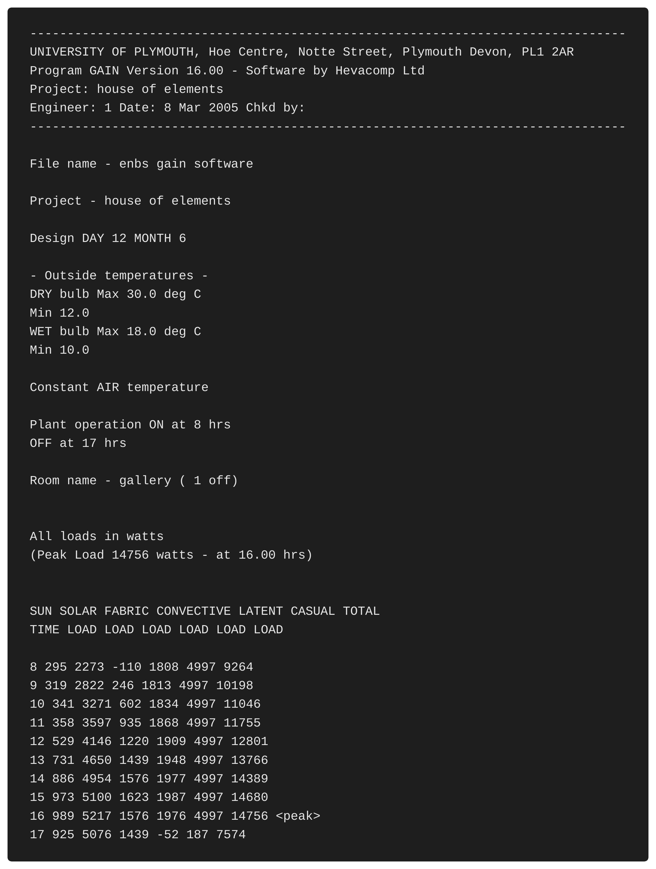
Table 17:
Summer hourly temperatures
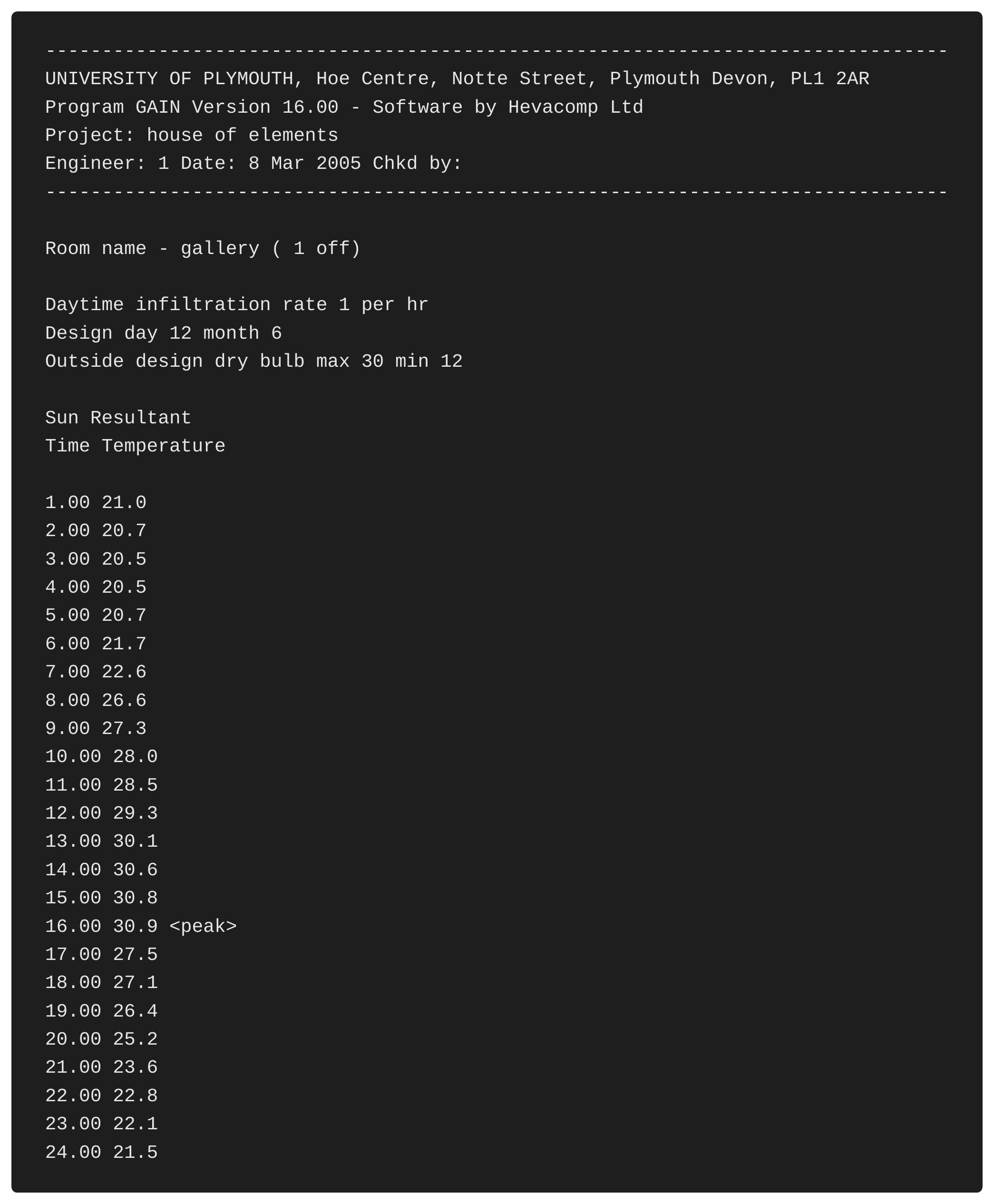
Table 18:
Solar azimuth and altitude:
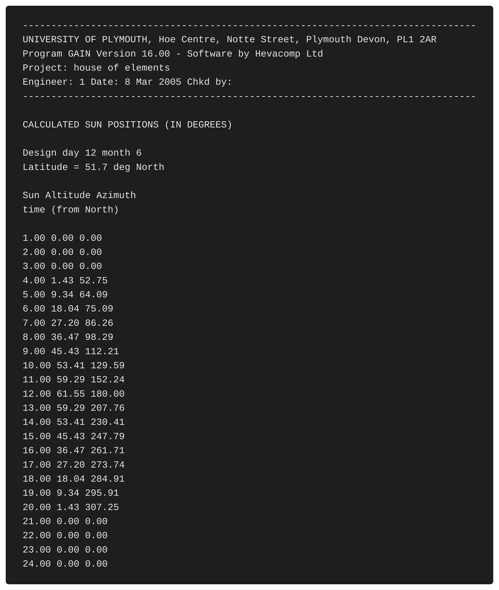
Table 19:
Shadow Angle Example:
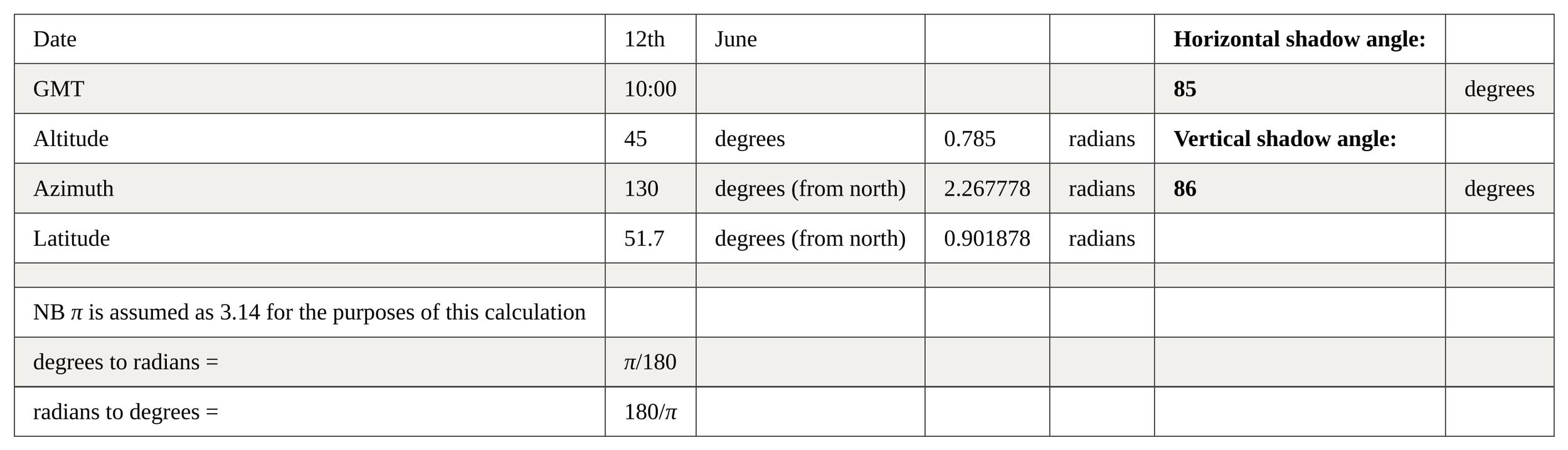
Conclusion
The effects that direct sunlight have upon a design are quite great, here is a list of effects that sunlight has upon a variety of designs (this is by no means comprehensive):
The entrance and exit of a garage – a driver would not want glaring sunlight in their eyes!
Dustbins should be shaded;
Larders and perishable foods need to be kept cool and shaded;
Art galleries must restrict amount of direct lighting upon paintings;
Libraries, protection of valuable manuscripts is a must;
Museums;
Laboratories – bacteria may need protection.
From “File 3. Solar geometry.xls” I have calculated that at 10am on a summers morning on June 16th the vertical shadow angle and horizontal shadow angle are 85º and 86º respectively. This is quite a steep angle but can be accounted for because the sun is very high in the sky in the summer, especially at ten in the morning. This has effected my design of my gallery because previously I had designed it to face south, this meant that too much sun would enter the building through the glazing, an could damage the art work on display. I had maximized glazing on the south side of my building and included none on the north side so as to take advantage of solar gain but have now decided against this. My gallery has been turned around and moved to a more shaded position, small north facing windows are included to provide daylight instead of sunlight for natural lighting. Also to prevent overheating and aid natural heating of the space a turf roof is used.
Final Conclusion
The Bedford Calidity is extremely useful to the designer because it incorporates all of the measurements of thermal comfort into one number. Using this set of calculations to calculate the Bedford calidity easily guides the designer to know if their room is too hot, too cool, too damp or too dry. A “perfect” Bedford Calidity is deemed to be around 4 ºC. This would include natural ventilation, a good internal temperature and not too much or too little condensation in the air.
In my opinion natural lighting should affect designs strongly, natural light is important within buildings, especially those that need this light for art work or drawing. For rooms such as workshops or studios the designer should attempt to put the areas that need the light the most as close to the windows as possible – natural lighting through a window is effective of up to 2 metres into the room (See L2), this number may change depending on the position and orientation of the building.
Artificial lights often cause colours to look different than they actually are, this difference is often so small that it is not noticed until the two different colour spectrums are compared side by side. As can be seen from my previous studies natural lighting is quite important for watercolours. When designing a room the specification of lights chosen should be studied carefully so that the desired effect is created.
A buildings position is often effected by the sun (see appendix 1), for example the position of my gallery, garden, greenhouse and internal courtyard (from my “House of the Elements” design project) has been positioned precisely to catch the sun. The gallery has been turned by 45 degrees so that too much sunlight will not enter the building and damage valuable art work, the courtyard is on a slight hill, with some walls dipped to allow extra sunlight in. My greenhouse has moved further north so that shadows cast by a cliff do not reduce the amount of sunlight it “catches” each year. Another effect that the sun has had upon my design is the inclusion of trees at strategic positions to provide solar shading (see appendix 1 & 3), I have used trees in a number of places on my design, but as of yet have not chosen on the final position for them. It is likely that they will be located near my greenhouse and garden to create some slightly sheltered areas for different types of plants. I believe that daylight, and especially sunlight should always have a strong influence upon a design, even if no sunlight is needed in the building it should still be investigated to check that it will cause no negative effects upon a design.
Skylight factors are really a theoretical measurement, especially when clouds are moving quickly as I have experienced! Because the amount of sun can rapidly change it is often quite difficult to measure the exact amount in a room, for this reason ASF% should be “taken with a pinch of salt” and only used as a guide, they are by no means a “true” calculation. The Sumpner‑Lynes‑Crisp method is probably one of the most important methods that designers should use, as discussed earlier it is extremely useful for calculating sunlight patches and shadows and should not be underestimated. I have been surprised by the amount of times I have considered sunlight, shadows, and daylight for my design (see appendix 1).
A designer should always be aware of any potential noise pollution and attempt to “design this out” rather than preventing it. For example rather than positioning a reading room next to a sports hall and including lots of sound insulation, simply change the design so that the reading room is not connected to the sports hall, maybe the changing rooms or a corridor divide them to help prevent unwanted noise. For my “House of the Elements” I have used this tactic to reposition my workshop and library so that noise does not cause a problem to the people in the library or meeting room adjacent. To move my workshop away slightly I included a cupboard/store and IT room – both of which will help prevent noise travelling between the areas.
If my building was near a main road or other source of noise I may consider moving quiet rooms to the back of my building or positioning trees to the front of the site; these would help to dampen unwanted sounds. As discussed traffic causes low pitch frequency noises, to prevent these a mass of earth or hill may help, also lifting the floors (floating floors) from the ground would stop noise transmitted through the building structure. If my design had more than one floor (which it doesn’t) I would need to take into account unwanted noise from floors above. These can be prevented by (again) using floating floor, or by simply using carpets and not a hard surface; such as floor boards or lino.
Where unwanted noise can not be prevented by repositioning the room, such as in an existing building that is being modified then air gaps in doors and windows should not be overlooked. As my previous experiments showed these seemingly small gaps decrease the sound insulation of a door greatly. Specially designed windows can now be purchased that help prevent noise transmission, however care should be taken when they are installed, it is no use using a “high tech” product if it is installed incorrectly it will provide no benefit to the occupier.
Bibliography
McMullan, R (1992) Environmental Science in Building, The MacMillan Press Ltd., London, UK;
ACOUSTICS in Education (1975) HMSO, Department of Education and Science, Building Bulletin 51;
Adler, David (1999) Metric Handbook, Planning and Design data, 2nd Edition. Architectural Press, UK
Appendix 1
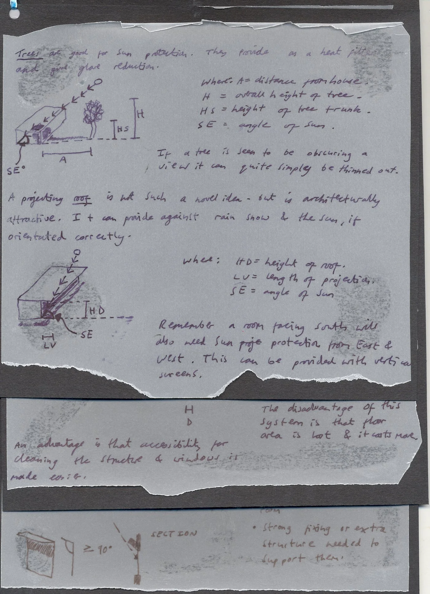
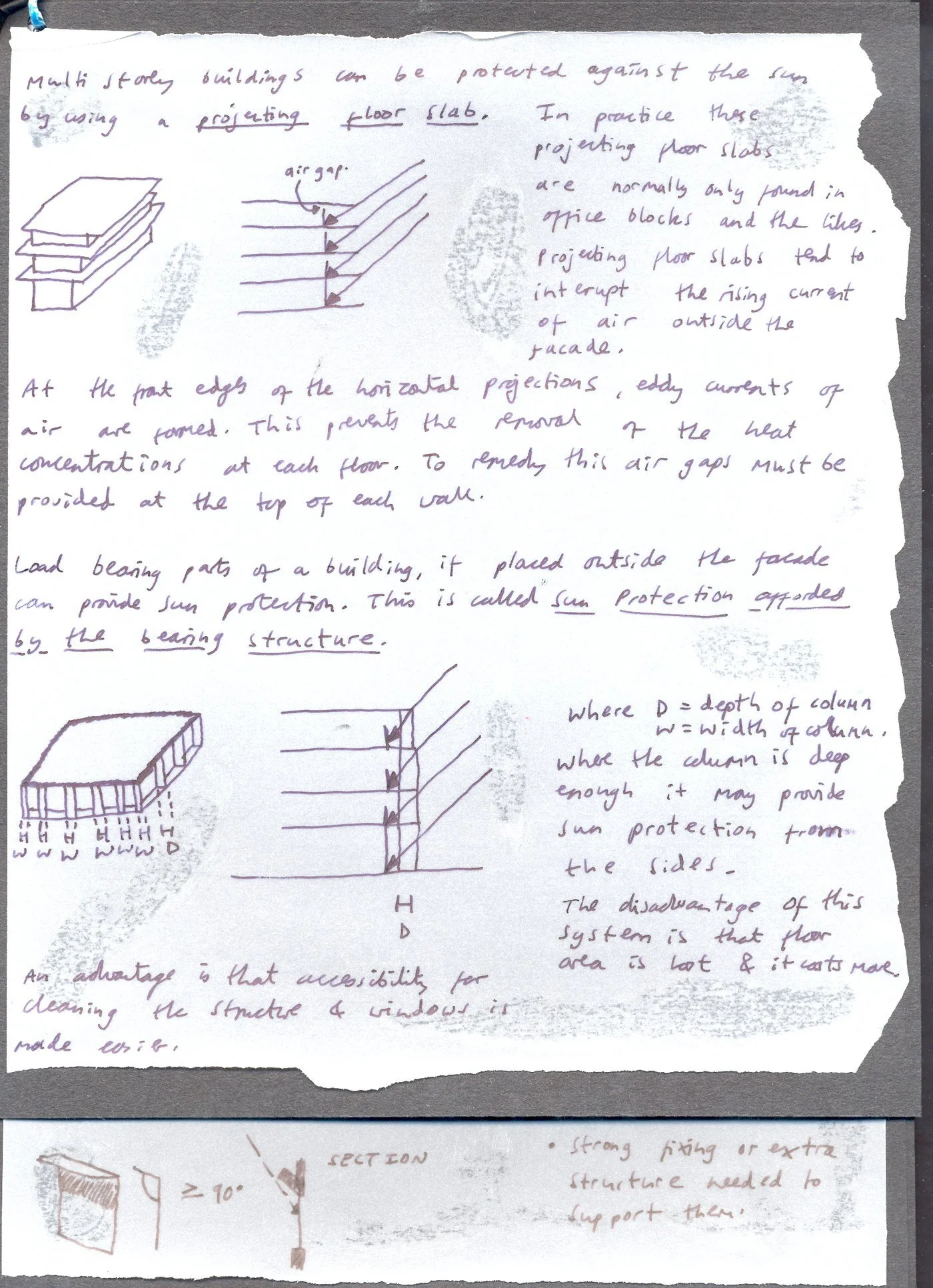
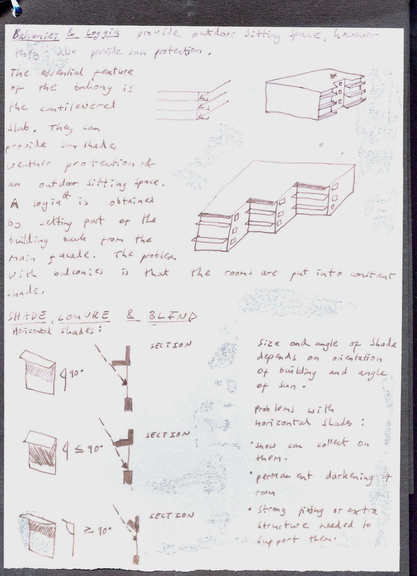
Appendix 2
Appendix 3
My “House of the Elements” design.
NB this design has been altered since (partially due to energetics calculations).
Line 1 shows the approximate line of the sun at the summer solstice
Line 2 shows the line at the middle of the solstices.
Line 3 shows the approximate line of the sun at the winter solstice
NB there is a Cliffside on 3 edges of my site that causes a large amount of shadow – hence the position of the “solar lines”.
Because of the lines (shadows) that the sun will create at the solstices I have pushed my greenhouse further north to be able to collect more sun. Also I have pointed my galleries to the north so they don’t let too much sunlight in (windows outlined with blue squiggle). The blue shading next to the bar and restaurant denotes a balcony or awning, this provides a buffer space for the north facing windows so that too much heat is not lost.
Notes & Sources
File 1. Module booklet 0405.doc – Part L1 – Admin Folder - Richard Griffiths.
File 2. Psychometric chart.doc – Information Folder – Richard Griffiths.
File 2. Psychometric chart.doc – Information Folder – Richard Griffiths.
File 0. Air velocity by kata sum.xls – Software Folder – Richard Griffiths.
File 1. Bedford Caladity calculation.xls – Software Folder – Richard Griffiths.
File 1. Module booklet 0405.doc – Admin Folder – Richard Griffiths.
File 1. Module booklet 0405.doc – Admin Folder – Richard Griffiths.
File 1. Module booklet 0405.doc – Part S1 – Admin Folder - Richard Griffiths.
File 2. Energy balance and ASF%.xls – Software Folder – Richard Griffiths.
File 1. Module booklet 0405.doc – Part L4 – Admin Folder - Richard Griffiths.
File 4. Noise in dB and dB(A).xls – Software Folder – Richard Griffiths.
File 1. Module booklet 0405.doc – Part L4 – Admin Folder - Richard Griffiths.
File 1. Module booklet 0405.doc – Part L4 – Admin Folder - Richard Griffiths.
File 4 Noise in dB and dB(A) – Software Folder – Richard Griffiths.
File 1. Module booklet 0405.doc – Part L4 – Admin Folder - Richard Griffiths.
File 8. Noise transmission.xls – Software Folder – Richard Griffiths.
RT ~ Reverberation Time.
File 1. Module booklet 0405.doc – Part S4 – Admin Folder - Richard Griffiths.
File 1. Module booklet 0405.doc – Part S4 – Admin Folder - Richard Griffiths.
ACOUSTICS in Education – HMSO, Department of Education and Science, Building Bulletin 51. 1975
File 1. Module booklet 0405.doc – Part S4 – Admin Folder - Richard Griffiths.
File 6 Acoustics RT, SRI and SPINY.xls – Software Folder – Richard Griffiths.
File 1. Module booklet 0405.doc – Part S4 – Admin Folder - Richard Griffiths.
File 6 Acoustics RT, SRI and SPINY.xls – Software Folder – Richard Griffiths.
See Table 10
File 1. Module booklet 0405.doc – Part S4 – Admin Folder - Richard Griffiths.
File 6 Acoustics RT, SRI and SPINY.xls – Software Folder – Richard Griffiths.
See Table 10
ASF% means Average Skylight Factor Percentage. This should not be confused with asf% which means Average Sunlight Factor Percentage.
File 1. Module booklet 0405.doc – Part L3 – Admin Folder - Richard Griffiths.
File 1. Module booklet 0405.doc – Part L3 – Admin Folder - Richard Griffiths.
File 1. Module booklet 0405.doc – Part L3 – Admin Folder - Richard Griffiths.
File 1. Module booklet 0405.doc – Part S3 – Admin Folder - Richard Griffiths.
File – Lighting.xls my ENBS diary Folder – Mark Ellery.
